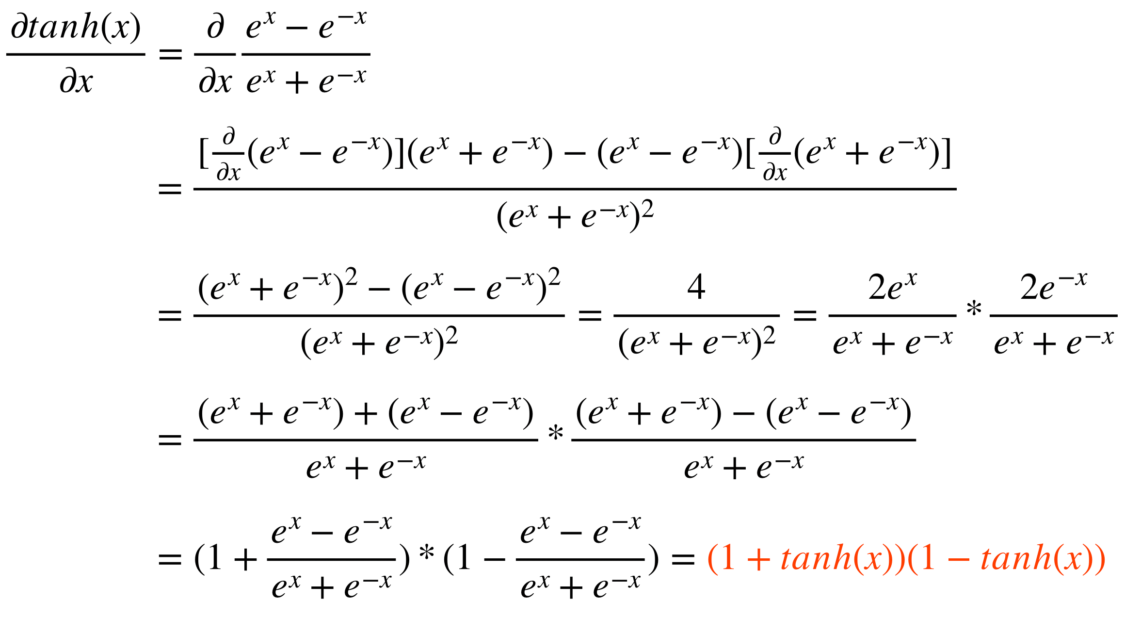
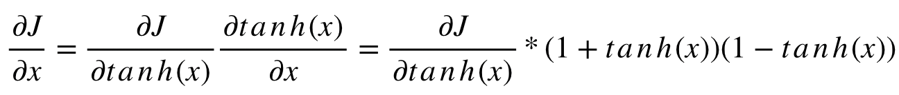
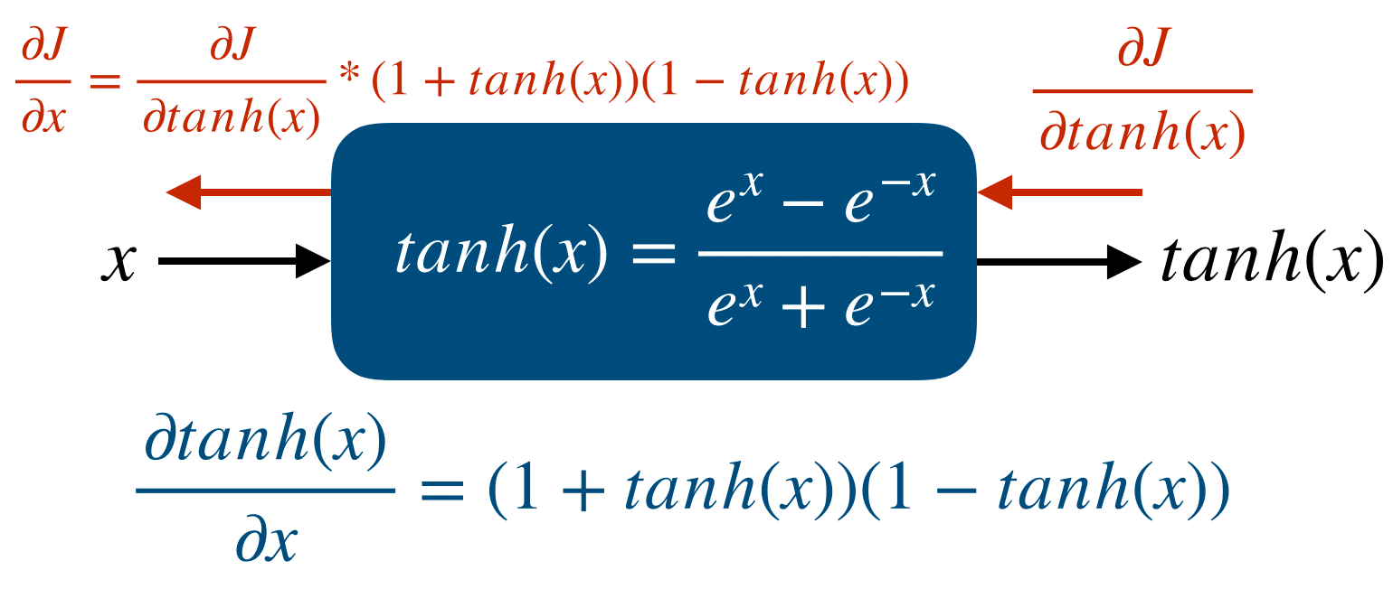
tf.GradientTape

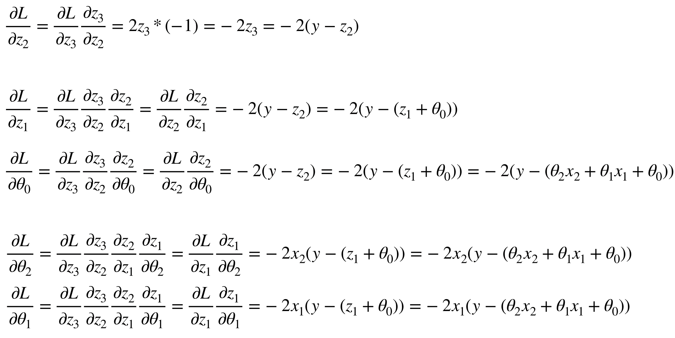
Neural network를 만든다는 것은 곧 computational graph를 만든다는 것이다. 즉 node와 edge를 만들어 network computation을 만든다. 일반적인 computational graph와는 다르게 deep learning에서는 prediction과 loss를 연산하는 forward propagation과 partial derivative와 vector chain rule을 이용한 backpropagation이 존재한다.


우리가 Tensorflow와 같은 deep learning framework를 이용하는 가장 큰 이유는 이 forward/backward propagation을 쉽게 구현할 수 있도록 도와주는 Automatic Differentiation 기능일 것이다. 이는 forward propagation에서 일어나는 모든 연산에 대해 gradient를 자동으로 저장해주고 이를 통해 gradient descent method를 쉽게 사용할 수 있게 해준다.


그리고 backpropagation을 연산할 때 하나하나 gradient를 구하는 것이 아니라 forward propagation이 진행될 때 이 값들을 저장해두면 backpropagation에서 이 저장된 값들을 이용하여 훨씬 빠르게 연산이 가능하다. 이때 tf.GradientTape에는 forward propagation이 진행되면서 나중에 backpropagation을 할 때 필요한 값들을 저장해둔다.


정리하면 이렇다. backpropagation을 할 때 forward propagation 값들을 저장해두면 이를 이용해 훨씬 빠르게 연산을 할 수 있다. 따라서 forward propagation이 진행되는 동안 그 값들을 저장할 필요가 있다. 즉, prediction을 구하는 과정과 loss를 구하는 과정이 tf.GradientTape의 대상이 되는 것이다.


tf.GradientTape Exmaple

이 gradient tape을 설명하는데 글로만 주구장창 말하는 것보다 예를 드는 것이 더 이해하기 쉬울 것 같아 예시를 들어보려고 한다.

test_list1 = [1, 2, 3]
test_list2 = [10, 20, 30]

t1 = tf.Variable(test_list1, dtype=tf.float32)
t2 = tf.Variable(test_list2, dtype=tf.float32)

with tf.GradientTape() as tape:
    t3 = t1 * t2

gradients = tape.gradient(t3, [t1, t2])
print(gradients[0])
'''
tf.Tensor([10. 20. 30.], shape=(3,), dtype=float32)
'''

print(gradients[1])
'''
tf.Tensor([1. 2. 3.], shape=(3,), dtype=float32)
'''

위에서는 variable tensor 2개를 만들고 gradient tape에서 이를 곱하는 t3를 만들었다. 그러면 Tensorflow는 t1, t2 node를 이용해 t3를 구하는 computational graph를 만든다. 그리고 이에 대한 연산값들을 저장한다.


그 뒤에 gradient를 구하는 과정은 tape.gradient이다. 첫 번째 t3는 target이므로 보통 loss가 된다. 그리고 그 뒤에는 우리가 학습시키려는 variable tensor를 넣어주면 된다. 이때 gradients[0]은 t3에 대한 t1의 gradient, gradients[1]는 t3에 대한 t2의 gradient가 된다.


위의 결과에서 알 수 있듯이, t3를 구하는데 t1과 t2를 element-wise로 곱했으므로 그 결과는 서로의 vector가 된다. 그 결과로 각자 이론과 동일한 결과를 얻을 수 있다.


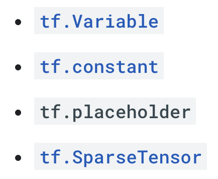
앞선 포스팅에서 Tensorflow에서 기본적인 tensor는 두 가지가 있다고 했고 이는 constant tensor와 variable tensor이다. 그리고 이들은 각각 input/label, trainable variable이 된다고 했다. 따라서 우리는 constant tensor에 대한 gradient를 구하는 것은 시간 낭비가 될 것이다. 다음 예제를 살펴보자.


test_list1 = [1, 2, 3]
test_list2 = [10, 20, 30]

t1 = tf.constant(test_list1, dtype=tf.float32)
t2 = tf.Variable(test_list2, dtype=tf.float32)

with tf.GradientTape() as tape:
    t3 = t1 * t2

gradients = tape.gradient(t3, [t1, t2])
print(gradients[0])
'''
None
'''

print(gradients[1])
'''
tf.Tensor([1. 2. 3.], shape=(3,), dtype=float32)
'''

위의 결과에서 t3에 대한 t1의 gradient는 구해지지 않았고 t2의 gradient는 구해졌다. 이처럼 Tensorflow는 학습이 필요없는 node에 대해서는 gradient가 구해지지 않음을 알 수 있다.


Simple Linear Regression Example

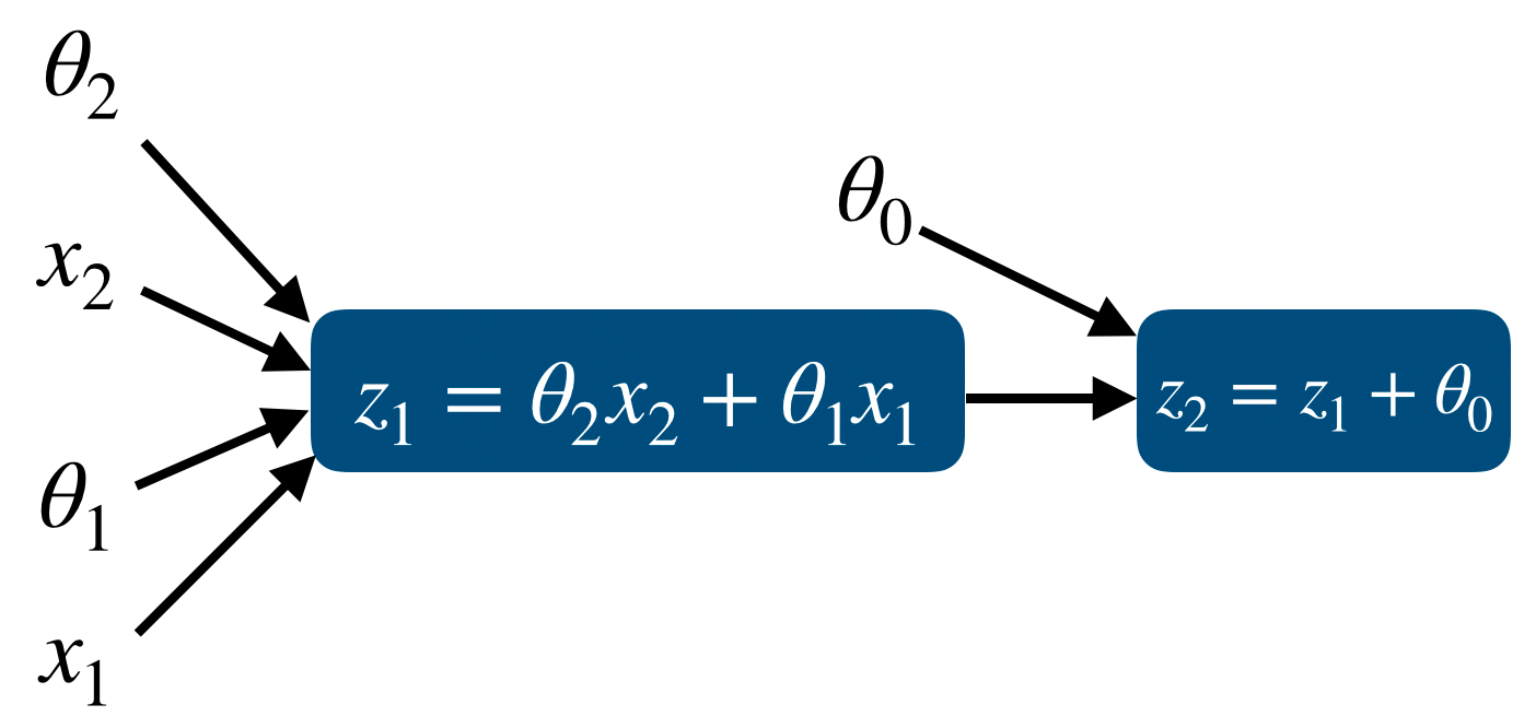
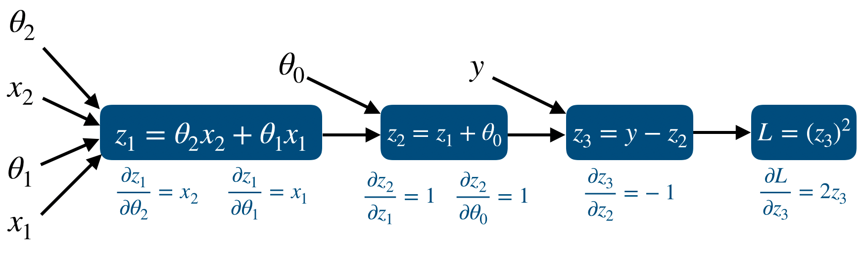
simple linear regression은 predictor가 y=wx + b인 regression이다. 따라서 weight, bias는 모두 1개이고 loss는 mean squared error를 사용한다. 이를 위한 toy dataset은 다음과 같이 tf.constant로 만들어줄 수 있다.

x_data = tf.constant([-1, -0.5, 0.5, 1], dtype=tf.float32)
y_data = 3*x_data + 1


학습을 위한 trainable parameter인 w, b는 다음과 같이 tf.Variable로 만들어준다

w = tf.Variable(-1.)
b = tf.Variable(-1.)

그리고 learning rate은 0.1로, w와 b의 변화를 추적하기 위한 w_trace, b_trace를 만들어준다.

LR = 0.1
w_trace, b_trace = [], []


그 후에 학습이 진행되는 코드는 다음과 같다.

for epoch in range(10):
    for x, y in zip(x_data, y_data):
        with tf.GradientTape() as tape:
            predictions = w*x + b
            loss = (predictions - y)**2
        gradients = tape.gradient(loss, [w, b])

        w = tf.Variable(w - LR*gradients[0])
        b = tf.Variable(b - LR*gradients[1])
        w_trace.append(w.numpy())
        b_trace.append(b.numpy())

위에서 알 수 있듯이 prediction과 loss를 계산하는 부분은 tf.GradientTape 안에 있다. 이때 backpropagation을 위한 값들이 저장되고, gradient는 w, b에 대해 구한다. 마지막으로 SGD를 이용하여 w, b를 update하면 된다.  그리고 w, b의 update되는 상태는 다음과 같다.

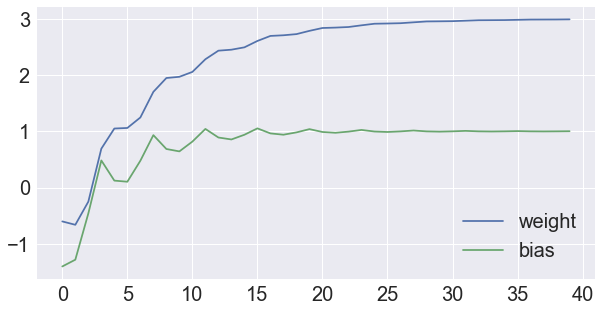
이처럼 tf.GradientTape은 forward propagation에 필요하다는 개념만 알면 이후에 오는 학습 코드들도 어렵지 않게 받아들일 수 있을 것이다.

Element-wise Operations in Tensorflow

Tensorflow의 tensor operation들은 NumPy의 영향을 크게 받았다. 그리고 NumPy에서 제공하는 ndarray 끼리의 사칙연산은 element-wise operation이다. 따라서 Tensorflow에서도 다음과 같은 연산결과를 얻을 수 있다.

t1 = tf.constant([10, 20, 30])
t2 = tf.Variable([1, 2, 3])

print(t1 + t2)
# tf.Tensor([11 22 33], shape=(3,), dtype=int32)

print(t1 - t2)
# tf.Tensor([ 9 18 27], shape=(3,), dtype=int32)

print(t1 * t2)
# tf.Tensor([10 40 90], shape=(3,), dtype=int32)

print(t1 / t2)
# tf.Tensor([10. 10. 10.], shape=(3,), dtype=float64)

print(t1 % t2)
# tf.Tensor([0 0 0], shape=(3,), dtype=int32)

print(t1 // t2)
# tf.Tensor([10 10 10], shape=(3,), dtype=int32)


Broadcasting Mechanism

Tensorflow의 tensor operation에 존재하는 broadcasting또한 NumPy의 broadcasting과 동일하게 작동한다.

위에서는 같은 수의 element를 가지는 vector들끼리의 operation이었다면 이번엔 다음과 같은 상황을 생각해보자.

t1 = tf.random.uniform(shape=(3, 4), minval=0, maxval=10)
t2 = tf.random.uniform(shape=(1, 4), minval=0, maxval=10)

print(t1.shape)
# (3, 4)

print(t2.shape)
# (1, 4)


수학적으로 이 두 matrices를 더하는 것은 정의되지 않는다. 하지만 우리는 scalar와 vector를 곱할 때 vector의 각 element마다 scalar를 곱해주는 것을 알고 있고, 이 개념을 이용한다면 t2라는 row vector를 t1에 row-wise로 더해주는 것이 자연스럽다고 느낄 수 있다.

실제로 많은 경우에 tensor operation을 할 때 shape을 맞춰주는 것은 어려운 것을 떠나 귀찮은 일이 된다. 이를 위해 Tensorflow는 broadcasting을 통해 이 자연스러운 연산을 진행한다.

t1 = tf.random.uniform(shape=(3, 4), minval=0, maxval=10)
t2 = tf.random.uniform(shape=(1, 4), minval=0, maxval=10)

t1 = tf.cast(t1, tf.int16)
t2 = tf.cast(t2, tf.int16)

print(t1.numpy())
'''
[[3 8 2 7]
 [5 6 3 9]
 [7 9 0 5]]
'''

print(t2.numpy())
'''
[[8 7 6 4]]
'''

print((t1 + t2).numpy())
'''
[[11 15  8 11]
 [13 13  9 13]
 [15 16  6  9]]
'''

위의 tf.cast는 data type을 바꿔주는 API이고 결과를 더 보기 쉽게 만들기 위해 사용했다.

결과에서 보이는 것처럼 t1은 (3, 4), t2는 (1, 4)였지만 t2를 (3, 4)로 broadcasting하여 연산을 진행했다. 이런 연산은 tabular data가 있고 각 data sample마다 일정한 연산을 해줄 때 매우 편리하다


broadcasting은 shape에 따라 기능이 달라지므로 다음의 연산에서는 위와 다른 결과가 나온다.

t1 = tf.random.uniform(shape=(3, 4), minval=0, maxval=10)
t2 = tf.random.uniform(shape=(3, 1), minval=0, maxval=10)

t1 = tf.cast(t1, tf.int16)
t2 = tf.cast(t2, tf.int16)

print(t1.numpy())
'''
[[3 2 8 3]
 [3 6 6 1]
 [0 9 2 8]]
'''

print(t2.numpy())
'''
[[6]
 [9]
 [7]]
'''

print((t1 + t2).numpy())
'''
[[ 9  8 14  9]
 [12 15 15 10]
 [ 7 16  9 15]]
'''

이번에는 t2가 (3, 1)이었으므로 coloumn-wise로 broadcasting되어 연산했다. 마지막으로 서로 row vector, column vector일 때의 연산은 다음과 같다.

t1 = tf.random.uniform(shape=(3, 1), minval=0, maxval=10)
t2 = tf.random.uniform(shape=(1, 4), minval=0, maxval=10)

t1 = tf.cast(t1, tf.int16)
t2 = tf.cast(t2, tf.int16)

print(t1.numpy())
'''
[[3]
 [6]
 [9]]
'''

print(t2.numpy())
'''
[[5 2 5 1]]
'''

print((t1 + t2).numpy())
'''
[[ 8  5  8  4]
 [11  8 11  7]
 [14 11 14 10]]
'''

위의 결과에서 알 수 있듯이 (3, 1)과 (1, 4)를 연산하기 위해서 모두 (3, 4)로 shape을 바꿔준 뒤 연산이 진행됐다. 이처럼 broadcasting을 잘 사용하면 for문을 이용할 필요없이 더 빠르고 쉽게 연산을 진행할 수 있다.


tf.reduce Family

tf에는 다양한 reduce API들이 있다. 먼저 나열해보면 다음과 같다.

  • tf.reduce_sum: element의 summation을 구함
  • tf.reduce_prod: element의 곱을 구함


  • tf.reduce_max: 최댓값 구함
  • tf.reduce_min: 최솟값 구함


  • tf.reduce_mean: 평균 구함
  • tf.reduce_std: 표준편차 구함
  • tf.reduce_variance: 분산 구함


  • tf.reduce_all: AND 연산
  • tf.reduce_any: OR 연산

위에 나열된 reduce family들은 기본적인 사용법이 동일하다. 따라서 대표로 tf.reduce_sum을 이용해 사용법을 살펴보자.


t1 = tf.random.uniform((3, 3), maxval=10, dtype=tf.int32)

print(t1.numpy())
'''
[[3 6 1]
 [1 8 4]
 [9 2 9]]
'''
print(tf.reduce_sum(t1).numpy())
'''
43
'''

위와 같이 tf.reduce_sum에 tensor만 넣어주면 모든 element의 합을 구해준다. 하지만 이런 경우보다는 axis를 설정해주는 경우가 많으므로 axis argument를 사용하는 방법에 대해 알아보자. 이 axis는 생각보다 헷갈려하는 사람이 많으므로 꼭 스스로 연습을 할 필요가 있다.


t1 = tf.random.uniform((2, 3), maxval=10, dtype=tf.int32)
print(t1.numpy())
'''
[[4 1 2]
 [0 4 3]]
'''

t2 = tf.reduce_sum(t1, axis=0)
print(t2.numpy())
'''
[4 5 5]
'''

위에서 보면 같은 column에 있는 값들을 모두 더한 것을 알 수 있다. 이를 다시 말하면 첫 번째 dimension인 2를 없앴다고 생각할 수 있다.  

우리의 data들은 보통 row에는 sample, column에는 attribute가 들어있다. 이때 모든 sample들에 들어있는 attribute값들을 더한게 바로 axis=0이라고 생각할 수 있다. 이때 알아둬야 할 점은 첫 번째 dimension을 기준으로 더했기 때문에 결과는 3개의 element를 가지는 vector가 된다.


반대로 axis=1로 설정하면 다음과 같다.

t1 = tf.random.uniform((2, 3), maxval=10, dtype=tf.int32)
print(t1.numpy())
'''
[[1 1 1]
 [7 2 1]]
'''

t2 = tf.reduce_sum(t1, axis=1)
print(t2.numpy())
'''
[ 3 10]
'''

이번엔 두 번째 axis를 기준으로 더했기 때문에 두 번째 dimension에 있는 값들을 모두 더한 것이다. 즉 data들이 각자 가지고 있는 attribute들의 합이 된다. 여기서도 마찬가지로 두 번째 dimension인 3을 기준으로 더했기 때문에 결과는 2개의 element를 가지는 vector가 된다.


이 개념을 확실히 다지기 위해 3차원 tensor를 이용해서 복습해보자.

t1 = tf.random.uniform((2, 3, 4), maxval=10, dtype=tf.int32)
print(t1.numpy())
'''
[[[4 3 5 8]
  [6 6 0 7]
  [3 2 5 8]]

 [[1 2 7 6]
  [4 8 1 3]
  [9 1 7 6]]]
'''

t2 = tf.reduce_sum(t1, axis=0)
print(t2.numpy())
'''
[[ 5  5 12 14]
 [10 14  1 10]
 [12  3 12 14]]
'''

t1이 (2, 3, 4)의 shape을 가지는 tensor일 때 axis=0으로 더해보면 결과는 (3, 4)가 된다. t1은 (3, 4)짜리 matrix를 두 개 곂쳐놨다고 생각할 수 있고, axis=0으로 더하면 이 두 행렬을 element-wise로 더했다고 생각할 수 있다. 여기서는 첫 번째 dimension 2를 기준으로 더했기 때문에 결과는 (3, 4)가 된다.


다음의 예제는 RGB channel을 가지는 128x128의 이미지를 다루는 예제이다.

t1 = tf.random.uniform((128, 128, 3), maxval=10, dtype=tf.int32)
print(t1.shape)
'''
(128, 128, 3)
'''

t2 = tf.reduce_sum(t1, axis=2)
print(t2.shape)
'''
(128, 128)
'''

위와 같이 t1이라는 이미지에 대해 channel에 있는 모든 값을 합하고 싶다면 axis=2로 설정해주면 된다. channel-wise로 더했기 때문에 결과는 128x128의 gray image가 되는 것이다. 물론 uint8을 넘어가겠지만 개념적으로는 그렇다.


위와 같이 axis에 대한 개념을 잘 잡았다면 나머지 tf.reduce family들은 사용방법이 동일하다.

Making High-Dimension Tensors

Data Science를 하다보면 element가 상당히 많은 tensor를 만들일이 많다. 이때 일일히 값을 넣어주려면 다음과 같은 문제가 발생한다.

test_list = [[1, 1, 1], [1, 1, 1], [1, 1, 1],
             [1, 1, 1], [1, 1, 1], [1, 1, 1],
             [1, 1, 1], [1, 1, 1], [1, 1, 1]]
t1 = tf.constant(test_list)
print(t1)

'''
tf.Tensor(
[[1 1 1]
 [1 1 1]
 [1 1 1]
 [1 1 1]
 [1 1 1]
 [1 1 1]
 [1 1 1]
 [1 1 1]
 [1 1 1]], shape=(9, 3), dtype=int32)
'''

단순히 모든 값이 1인 9x3의 matrix를 만드는데에도 이런 노력이 필요하다. 나아가 특정한 random distribution에서부터 random value들을 가지는 tensor를 만들기 위해서는 Numpy의 np.random을 사용해야 한다.


이를 해결하기 위해 Tensorflow는 NumPy와 거의 동일한 API들을 제공한다. 물론 NumPy에서 같은 기능을 하는 API를 통해 ndarray를 만들고 tf.constant, tf.Variable, tf.conver_to_tensor를 이용해 Tensorflow의 tensor를 만들어줘도 된다.


tf.ones / tf.ones_like

위의 예제를 쉽게 해결해주는 tf.ones가 있다. 이는 NumPy와 사용법이 동일하다.

t2 = tf.ones(shape=(9, 3))
print(t1)
'''
tf.Tensor(
[[1. 1. 1.]
 [1. 1. 1.]
 [1. 1. 1.]
 [1. 1. 1.]
 [1. 1. 1.]
 [1. 1. 1.]
 [1. 1. 1.]
 [1. 1. 1.]
 [1. 1. 1.]], shape=(9, 3), dtype=float32)
'''

위의 tf.ones를 이용하면 고차원의 tensor도 쉽게 만들수가 있다. 이 ones API를 처음보는 사람이면 별거 없어 보이겠지만, 실제 프로그래밍을 하다보면 상당히 많이 사용된다. 따라서 독자들은 꼭 잘 숙지하고 넘어갔으면 한다. 참고로 눈치빠른 독자라면 위의 tensor는 1로 채워져있는데 data type이 float32인 것을 알 것이다. 이는 Tensorflow에서는 기본적인 tensor의 data type이 float32이기 때문이다.


뒤에서 다룰 tensor operation의 내용을 조금 빌려오자면, 다른 값을 가지는 tensor도 tf.ones를 이용해 쉽게 만들 수 있다.

t3 = 3.*tf.ones(shape=(3, 3))
print(t3)
'''
tf.Tensor(
[[3. 3. 3.]
 [3. 3. 3.]
 [3. 3. 3.]], shape=(3, 3), dtype=float32)
'''
t4 = -tf.ones(shape=(3, 3))
print(t4)
'''
tf.Tensor(
[[-1. -1. -1.]
 [-1. -1. -1.]
 [-1. -1. -1.]], shape=(3, 3), dtype=float32)
'''
t5 = 3.14*tf.ones(shape=(3, 3))
print(t5)
'''
tf.Tensor(
[[3.14 3.14 3.14]
 [3.14 3.14 3.14]
 [3.14 3.14 3.14]], shape=(3, 3), dtype=float32)
'''

이 tf.ones를 잘 사용하면 굳이 tf.fill을 사용할 필요가 없게 된다. 


이어서 tf.ones_like는 ones_like는 이름에서 알 수 있듯이, 특정 tensor와 비슷하면서 모든 element가 1인 tensor를 만들어준다. 이때 '비슷하다'는 말은 shape을 말한다. 바로 예제를 살펴보자.

t1 = 3.14*tf.ones(shape=(3, 3))
print(t1)
'''
tf.Tensor(
[[3.14 3.14 3.14]
 [3.14 3.14 3.14]
 [3.14 3.14 3.14]], shape=(3, 3), dtype=float32)
'''

t2 = tf.ones_like(t1)
print(t2)
'''
tf.Tensor(
[[1. 1. 1.]
 [1. 1. 1.]
 [1. 1. 1.]], shape=(3, 3), dtype=float32)
'''

t1의 shape이 (3, 3)이었으므로 t2의 shape도 (3, 3)이 된다. 그러면서 모두 1로 채워주는 API가 tf.ones_like이다.


위의 tf.one와 tf.ones_like들은 다음에 배울 tf.zeros, tf.zeros_like와 마찬가지로 기본적인 딥러닝 network를 만들고 학습을 시키는데는 사실 필요없을 수도 있다. 하지만 조금만 수준이 높아지더라도 custom loss function을 만드는 등 이런 기능들은 적극적으로 사용된다.


tf.zeros / tf.zeros_like

tf.ones, tf.ones_like를 잘 봤다면 이름만 봐도 tf.zeros, tf.zeros_like API들은 어떻게 사용할지 감이 잡힐 것이다. 따라서 간단히 예시만 보고 넘어가도록 하자.

t1 = tf.zeros(shape=(5, 5))
print(t1)
'''
tf.Tensor(
[[0. 0. 0. 0. 0.]
 [0. 0. 0. 0. 0.]
 [0. 0. 0. 0. 0.]
 [0. 0. 0. 0. 0.]
 [0. 0. 0. 0. 0.]], shape=(5, 5), dtype=float32)
'''


t1 = 3.14*tf.ones(shape=(3, 3))
print(t1)
'''
tf.Tensor(
[[3.14 3.14 3.14]
 [3.14 3.14 3.14]
 [3.14 3.14 3.14]], shape=(3, 3), dtype=float32)
'''

t2 = tf.zeros_like(t1)
print(t2)
'''
tf.Tensor(
[[0. 0. 0.]
 [0. 0. 0.]
 [0. 0. 0.]], shape=(3, 3), dtype=float32)
'''


tf.random Module

Tensorflow의 random module이 가지고 있는 API들은 NumPy의 random module보다 그 수가 적다. 하지만 random seed를 설정하는 기능이나 random distribution에서 random value를 생성하는 과정은 동일하다.


사실 global generator와 같이 더 심도있게 배우면 좋은 것들이 많지만 이 포스팅에선 기본적인 random module의 사용법을 다룬다. 하지만 왠만하면 이 기능들로도 프로그래밍하는데 큰 어려움은 없을 것이다.


tf.random.set_seed

tf.random.set_seed는 random seed를 설정해주는 역할을 한다. 컴퓨터는 사실 실제로 random한 값들을 만들 수 없고, random seed를 이용해 이를 모사한 값들을 만들게 된다. 이때 random seed를 설정해주면 random한 상황을 일정하게 통제할 수 있게 된다. 이는 같은 random한 상황에서의 반복적인 테스트를 할 때 유용하게 사용된다.


random seed의 효과를 비교하기 위해 먼저 다음과 같이 random value들을 생성해보자.

print(tf.random.normal((3, )))
# tf.Tensor([-1.8041286  -0.11153453 -0.845551  ], shape=(3,), dtype=float32)

print(tf.random.normal((3, )))
# tf.Tensor([ 1.698977  -0.7732199  0.2774948], shape=(3,), dtype=float32)

print(tf.random.normal((3, )))
# tf.Tensor([ 1.61399    2.4495301 -1.1530102], shape=(3,), dtype=float32)

위에서 알 수 있듯이 각 실행마다 마치 정말 random한 값들이 normal distribution에서부터 나오는 것을 알 수 있다. 그럼 random seed를 설정하고 다시 실행해보자.


tf.random.set_seed(0)
print(tf.random.normal((3, )))
# tf.Tensor([ 1.5110626   0.42292204 -0.41969493], shape=(3,), dtype=float32)

tf.random.set_seed(0)
print(tf.random.normal((3, )))
# tf.Tensor([ 1.5110626   0.42292204 -0.41969493], shape=(3,), dtype=float32)

tf.random.set_seed(0)
print(tf.random.normal((3, )))
# tf.Tensor([ 1.5110626   0.42292204 -0.41969493], shape=(3,), dtype=float32)

이번엔 모두 같은 결과가 나온 것을 알 수 있다. 이처럼 random effect를 무시한 reproducibility를 보장하기 위한 방법으로 다양한 경우에 random seed를 설정해준다. 이때 seed는 마음에 드는 숫자를 넣어주면 된다.


tf.random.normal

random distribution에서 가장 많이 사용되는 distribution은 아무래도 normal distribution일 것이다. 그리고 그 중에서도 mean, standard deviation이 각각 0, 1인 standard normal distribution은 다양한 경우에 사용된다. 따라서 가장 기본적인 tf.randon.normal의 사용법은 다음과 같이 standard normal distribution이 된다.

https://www.tensorflow.org/api_docs/python/tf/random/normal


random_data = tf.random.normal(shape=(3000, ))

fig, ax = plt.subplots(figsize=(10, 10))
ax.hist(random_data.numpy(),
        bins=30)
ax.tick_params(labelsize=20)

위의 결과에서 볼 수 있듯이 standard normal distribution에서 뽑힌 3000개의 sample들은 실제 standard normal distribution에 가깝다. 여기서 mean과 std를 바꿔주는 방법은 위의 document와 같이 mean, stddev를 바꿔주는 것이다.

random_data = tf.random.normal(shape=(3000, ),
                               mean=3, stddev=3)

fig, ax = plt.subplots(figsize=(10, 10))
ax.hist(random_data.numpy(),
        bins=30)
ax.tick_params(labelsize=20)

예상한 결과가 나오는 것을 알 수 있다. 물론 tf.random.set_seed를 쓴 뒤 위의 코드를 돌리면 항상 같은 결과가 나오게 된다.


tf.random.uniform / tf.random.possion / tf.random.gamma

각각의 distribution들은 argument만 다를 뿐 기본 사용법은 동일하므로 예제를 하나씩만 확인하고 가자

random_data = tf.random.uniform((3000, ),
                                minval=-5, maxval=5)
fig, ax = plt.subplots(figsize=(10, 10))
ax.hist(random_data.numpy(),
        bins=30)
ax.tick_params(labelsize=20)

random_data = tf.random.poisson((3000, ),
                                lam=5)
fig, ax = plt.subplots(figsize=(10, 10))
ax.hist(random_data.numpy(),
        bins=30)
ax.tick_params(labelsize=20)


random_data = tf.random.gamma((3000, ),
                              alpha=3)
fig, ax = plt.subplots(figsize=(10, 10))
ax.hist(random_data.numpy(),
        bins=30)
ax.tick_params(labelsize=20)


Tensors in Tensorflow

Tensorflow를 배우기 위해 알아야할 기본적인 tensor는 두 가지가 있다. 바로 아래의 4가지 중에 tf.Variable과 tf.constant이다.

https://www.tensorflow.org/guide/tensor?hl=ko

위의 두 가지 tensor는 각각 사용하는 용도가 다른데, tf.constant는 이름에서 알 수 있듯이 immutable object이다. 즉 내용 수정이 불가능하므로 학습에 필요한 input, label등에 사용될 수 있다. 단순히 immutable의 차이점이 아니라 우리가 딥러닝을 이용하여 학습을 진행할 때 input, label에 대한 학습은 할 필요가 없기 때문에 gradient가 자동으로 구해지지 않는 역할도 한다. 


한편 tf.Variable은 mutable object이다. 즉 내용의 값들이 바뀔 수 있고 training model의 weight, bias과 같은 trainable parameter는 iteration이 일어나면서 값이 바뀌어야 하므로 mutable object여야 한다. 추가적으로 학습 중 이 tf.Variable로 만들어진 object들은 gradient가 구해지고 이를 통해 값을 update할 수 있게 된다.


위의 차이점을 통해 Tensorflow 입문자들은 쉽게 dataset은 tf.constant, trainable parameter는 tf.Variable이라고 생각해도 큰 지장이 없다. 


Making Tensors in Tensorflow

글쓴이는 대부분의 Tensorflow 이용자들과 같이 Python 위에서 Tensorflow를 사용한다. Python 위에서 Tensorflow가 돌아가기 위해선 기존 Python primitive objects(예를 들어 Python list, string, number)들을 Tensorflow의 tensor로 만들어주는 API가 있으면 좋을 것이다. 당연히 Tensorflow는 이런 API들을 제공한다.


또한 data science에서 가장 많이 사용하는 data type은 Numpy array(ndarray)이다. 실제로 Tensorflow나 Pytorch의 tensor들은 모두 ndarray와 많이 닮아있다. 그래서 많은 tensor에 대한 operation들이 tf.를 np.로만 바꿔줘도 동작한다. 또한 OpenCV, Scikit-learn, Matplotlib과 같은 다양한 library들이 기존에 ndarray와 서로 공생관계에 있었으므로 Tensorflow도 ndarray로 부터 tensor를 만드는 API를 제공한다. 그리고 반대의 API도 물론 존재한다.


위와 같이 Tensorflow의 사용성을 확장하기 위해 Tensorflow에서는 tensor를 만드는 방법은 크게 세 가지

  • tf.constant
  • tf.convert_to_tensor
  • tf.Variable

가 있는데 이들은 모두 Python list, ndarry에서 tensor를 만들어낼 수 있다. 간단한 비교를 하고 살펴보도록 하자.

t1 = tf.constant([1, 2, 3])
t2 = tf.convert_to_tensor([1, 2, 3])
t3 = tf.Variable([1, 2, 3])

위에서 볼 수 있듯이 모두 Python list에서부터 tensor를 만들어낼 수 있고 arguemtn에 Python list나 ndarray를 넣어주면 된다. 각각의 tensor들을 출력해보면 다음과 같다


print(t1)
# tf.Tensor([1 2 3], shape=(3,), dtype=int32)
print(t2)
# tf.Tensor([1 2 3], shape=(3,), dtype=int32)
print(t3)
# <tf.Variable 'Variable:0' shape=(3,) dtype=int32, numpy=array([1, 2, 3], dtype=int32)>

t1, t2 tensor들은 서로 같은 결과가 나왔다. 즉, tf.constant와 tf.convert_to_tensor의 output은 같은 object라는 뜻일 것이다.

그리고 tf.Variable은 조금 다른 모습을 보이는 것을 알 수 있다. 그러면 각각의 data type을 출력해보자.


print(type(t1))
# <class 'tensorflow.python.framework.ops.EagerTensor'>
print(type(t2))
# <class 'tensorflow.python.framework.ops.EagerTensor'>
print(type(t3))
# <class 'tensorflow.python.ops.resource_variable_ops.ResourceVariable'>

예상한대로 tf.constant, tf.convert_to_tensor는 같은 object이고 tf.Variable은 다른 것을 알 수 있다. 이때 각각 EagerTensor, ResourceVariable이라는 클래스의 instant인 것을 확인할 수 있는데 이 타입에 따라 작동하는 방법이 달라지게 된다. 그럼 하나씩 살펴보자.


tf.constant

tf.constant의 argument에 Python list와 ndarray를 입력하면 다음과 같이 결과는 동일한 것을 알 수 있다. 즉 Python list와 ndarray를 가지고 Tensorflow의 constant tensor를 만들어낼 수 있다.

test_list = [1, 2, 3]
test_np = np.array([1, 2, 3])

t1 = tf.constant(test_list)
t2 = tf.constant(test_np)

print(t1)
# tf.Tensor([1 2 3], shape=(3,), dtype=int32)
print(t2)
# tf.Tensor([1 2 3], shape=(3,), dtype=int64)


추가적으로 다음을 통해서 constant tensor로부터 constant를 만들어낼 수 있는 것도 알 수 있다.

t3 = tf.constant(t1)
print(t3)
# tf.Tensor([1 2 3], shape=(3,), dtype=int32)


tf.Variable

tf.constant와 마찬가지로 tf.Variable에 Python list, ndarray를 이용하여 variable tensor를 만들어낼 수 있다. 이때 주의해야될 점은 tf.constant는 method이므로 소문자 c로 시작하고 tf.Variable은 클래스로부터 instance를 만들어내기 때문에 대문자 V로 시작한다. 이는 PEP8 convention을 따른 결과이다. 

test_list = [1, 2, 3]
test_np = np.array([1, 2, 3])

t1 = tf.Variable(test_list)
t2 = tf.Variable(test_np)

print(t1)
# <tf.Variable 'Variable:0' shape=(3,) dtype=int32, numpy=array([1, 2, 3], dtype=int32)>
print(t2)
# <tf.Variable 'Variable:0' shape=(3,) dtype=int64, numpy=array([1, 2, 3])>


추가적으로 다음을 실행시켜도 오류가 뜨지 않는다. 즉, constant tensor와 variable tensor를 모두 variable tensor로 만들 수 있다는 뜻이다. 이는 다음의 tf.convert_to_tensor를 설명하기 위해 미리 설명한다.

t3 = tf.constant(test_list)
t4 = tf.Variable(test_list)

t5 = tf.Variable(t3)
t6 = tf.Variable(t4)


tf.convert_to_tensor

마지막으로 tf.convert_to_tensor를 살펴보면 결과는 Python list, ndarray로부터 EagerTensor를 만들어내므로 동일한 API라고 생각할 수 있다. 하지만 다음의 코드를 실행시켜보면 오류가 발생하는 것을 알 수 있다.

test_list = [1, 2, 3]

t1 = tf.Variable(test_list)
t2 = tf.constant(t1)
# ValueError: TypeError: object of type 'ResourceVariable' has no len()


하지만 같은 과정을 tf.convert_to_tensor를 이용하면 다음과 같이 정상적으로 작동하는 것을 알 수 있다.

test_list = [1, 2, 3]

t1 = tf.Variable(test_list)
t2 = tf.convert_to_tensor(t1)


그럼 variable tensor를 constant tensor로 마음껏 바꿀 수 있을까?

test_list = [1, 2, 3]

t1 = tf.constant(test_list)
t2 = tf.Variable(t1)

위의 코드는 정상적으로 작동한다


여기서 '왜 이렇게 복잡하게 만들었을까?' 라는 질문이 생긴다. 이에 대해 글쓴이는 다음과 같이 추측한다.

딥러닝에서 학습을 시작할 때 trainable parameter를 initialization할 때를 제외하곤 크게 trainable parameter에 특정 값을 직접적으로 넣어줄 일이 없다. 이때는 variable이나 constant이나 initialization을 할 땐 크게 상관이 없다.

하지만 딥러닝 중에 variable을 다른 module에 전달해주는 경우는 많아도 아예 constant로 만들어버리는 경우는 많지 않다. 이 때문에 Tensorflow 개발자들이 실수를 방지하기 위함이 아닐까 생각한다.


물론 이 실수 하나 때문에 API를 만들진 않았을 것이다. 실제로 다양한 개발자들이 이 convert_to_tensor를 이용해 중간중간 tensor operation에 대한 custom function을 만들고 학습을 진행한다. 딱 이 이유 하나 때문은 아니겠지만 독자들은 이 차이점은 꼭 알고 넘어갔으면 좋겠다.


이상으로 이번 포스팅을 마치도록 한다.

Linear Model Simplification


Backpropagation for Binary Cross Entropy


Node

Partial Derivative

Chain Rule

Backpropagation

Simgoid Activation Funcion


Node

Partial Derivatives

Chain Rule

Backpropagation


Tanh Activation Funcion


Node

Partial Derivatives

Chain Rule

Backpropagation


ReLU Activation Funcion


Node

Partial Derivatives

Chain Rule

Backpropagation

이번 포스트에서는 Deep Learning에서 가장 많이 사용되는 activation function들인 sigmoid, tanh, ReLU에 대해서 알아본다.

실제로는 상당히 다양한 종류의 activation function들이 존재하고 2017년 Google Brain에서 개발한 Swish activation function 등, 지금도 효유적인 backpropagation을 위한 activation function들이 개발되고 있다.

이때 이 모든 activation function들을 한 번에 다루는 것은 비효율적이기도 하고, 지겨우니까 대표적인 activation function들에 대해 배우고, learning process에 접목시켜본 뒤에 다른 activation function들의 특징을 파악하는 편이 더 좋을 것 같다.


따라서 몇 차례의 포스트를 걸쳐 기본적인 sigmoid, tanh, ReLU에 대해서 배워보도록 하자.


Sigmoid Activation Function


Deep learning을 배우는 사람들은 아마 logistic regression을 배우면서 처음 sigmoid라는 non-linear activation function을 접할 것이다. 그리고 이 sigmoid function은 logistic function의 subset인데 output이 0과 1사이이므로 확률로의 해석이 가능하며 x축으로의 bias가 없어서 learning에 효과적이므로 logistic funciton들 중 가장 많이 사용된다.


먼저 logistic function의 식은 다음과 같다.

이 logistic function에서 input의 boundary를 (0,1)로 맞추고 x축에 대한 bias도 없애면

우리가 알고있는 sigmoid function의 형태가 된다. 이 sigmoid function는 함수의 모양과 도함수를 그려보면 다음과 같다.

x_range = np.linspace(-5, 5, 300)
sigmoid = 1 / (1 + np.exp(-1*x_range))
sigmoid_d = sigmoid*(1 - sigmoid)

fig, ax = plt.subplots(2, 1, figsize = (15,10))
ax[0].set_title("Sigmoid Function", fontsize = 20)
ax[0].plot(x_range, sigmoid)
ax[0].grid()

ax[1].set_title("Derivative of Sigmoid", fontsize = 20)
ax[1].plot(x_range, sigmoid_d)
ax[1].grid()


극한을 이용하여 sigmoid의 수렴값을 구해보면

이므로 sigmoid의 output은 확률로 해석이 가능하며

전체 0부터 1사이의 output 중 90% 정도인 0.1과 0.9를 input이 실수 전체 중 -2부터 2일때가 차지한다. 따라서 [-2, 2] 이외의 값들은 outlier로 취급되어 sigmoid의 output에서는 0.1, 0.9와 큰 차이를 보이지 않는다.


그리고 이 sigmoid의 derivative는 다음과 같이 구할 수 있다.


따라서 sigmoid function에 대한 node는 다음과 같이 구현할 수 있다.

class sigmoid_node():
    def __init__(self):
        self.x, self.z = None, None
        
    def forward(self, x):
        self.x = x
        self.z = 1 / (1 + np.exp(-1*self.x))
        return self.z
    
    def backward(self, dJ):
        return self.z * (1 - self.z) * dJ


Tanh Activation Fucntion


위의 sigmoid보다 대부분의 경우에서 좋은 성능을 보여주는 activation function은 tanh이다. 따라서 hidden layer에서 sigmoid보다 tanh를 사용하는 경우가 많다. 하지만 마지막 layer에서 classification을 할 때는 tanh보다 sigmoid를 많이 사용한다.

이 tanh activation function은 다음과 같다.


이 tanh의 모양과 도함수의 모양은 다음과 같다.

x_range = np.linspace(-5, 5, 300)
tanh = (np.exp(x_range) - np.exp(-1*x_range))/(np.exp(x_range) + np.exp(-1*x_range))
tanh_d = (1 + tanh)*(1 - tanh)

fig, ax = plt.subplots(2, 1, figsize = (15,10))
ax[0].set_title("Tanh Function", fontsize = 20)
ax[0].plot(x_range, tanh)
ax[0].grid()

ax[1].set_title("Derivative of Tanh", fontsize = 20)
ax[1].plot(x_range, tanh_d)
ax[1].grid()

위의 식에서 극한을 이용하면 다음과 같은 결과를 얻을 수 있다.


이때 알 수 있는 것은, sigmoid와 달리 activation function의 output이 zero-centered라는 것이다. 즉, deep learning의 hidden layer에 이 tanh를 사용할 경우, 다음 layer의 input이 자동으로 zero-centered input이 되는 것을 알 수 있다. 이것이 tanh가 sigmoid보다 좋은 성능을 보여주는 첫 번째 이유가 된다.


sigmoid와 마찬가지로 tanh의 도함수를 구해보면 다음과 같다.


따라서 tanh는 다음과 같이 구현할 수 있다.

class tanh_node():
    def __init__(self):
        self.x, self.z = None, None
    
    def forward(self, x):
        self.x = x
        self.z = (np.exp(self.x) - np.exp(-1*self.x))/(np.exp(self.x) + np.exp(-1*self.x))
        return self.z
        
    def backward(self, dJ):
        return (1 + self.z) * (1 - self.z) * dJ


ReLU Activation Function


요즘 deep learning에서 가장 첫 번째로 시도되는 activation function은 ReLU일 것이다. 이 ReLU가 다른 activation function보다 좋은 성능을 내는지에 대한 논문도 다양하며 실제로 다양한 neural network에서 좋은 성능을 보여준다. 먼저 ReLU의 식은 다음과 같다.


즉, ReLU의 input이 양수일 경우엔 그 양수값을 내보내고, 음수일 경우 0을 내보낸다. ReLU가 좋은 성능을 내는 첫 번째 이유가 이 식에 있다. Sigmoid, Tanh는 여러 연산들을 하여 activation value를 만드는데 비해, 이 ReLU는 한 번의 비교연산만을 통하여 output을 내기 때문에 연산속도가 빠르다. 보통 tanh보다 5배정도 빠르다고 알려져있다.


이 ReLU의 그래프와 도함수를 보면 다음과 같다.

x_range = np.linspace(-5, 5, 300)
zero_arr = np.zeros_like(x_range)
relu = np.maximum(x_range, zero_arr)
relu_d = relu / (0.0001 + relu)
fig, ax = plt.subplots(2, 1, figsize = (15,10))
ax[0].set_title("Tanh Function", fontsize = 20)
ax[0].plot(x_range, relu)
ax[0].grid()

ax[1].set_title("Derivative of Tanh", fontsize = 20)
ax[1].plot(x_range, relu_d)
ax[1].grid()

이때, 코드를 보면 relu_d를 구현하는데 조금의 트릭이 들어간 것을 알 수 있다. 음수일 때 0, 양수일 때 1을 만들기 위하여 relu에 relu를 나눠주는데 0으로 나눠줄 수 없으므로 gradient에 영향을 주지 않는 0.0001 정도를 더해서 나눠준 것을 알 수 있다.


도함수는 어렵게 구할 것 없이, 양수일 때는 1이고 음수일 때는 0이 된다.


따라서 ReLU는 다음과 같이 구현할 수 있다.

class relu_node():
    def __init__(self):
        self.x, self.z = None, None
        
    def forward(self, x):
        self.x = x
        self.z = np.maximum(0, self.x)
        return self.z
    
    def backward(self, dJ):
        return self.z / (0.0001 + self.z)

Activation Functions Comparison


위의 3가지 activation function을 같이 그려보면 다음과 같다.

먼저 위의 그래프를 통해 알 수 있는 것은, sigmoid와 tanh는 output의 범위가 정해져있지만 ReLU는 output의 범위가 정해져있지 않다는 것이다.

그리고 도함수에서 sigmoid와 tanh는 1보다 작기 때문에 layer가 많아질수록 propagate되는 값들이 0에 가까워질 것을 알 수 있다. 즉, sigmoid와 tanh는 태생적으로 vanishing gradient problem을 야기할 수 있는 activation function들이다.

마지막 Linear Regression에 대한 Backpropagtion으로 Multivariate Linear Regression에 대한 Backpropagation 정리노트이다.


Backpropagation for One Sample


Model

Parital Derivative

Chain Rule

Backpropagation Visualization

Parameter Update


Backpropagation for Two Samples


Model

Parital Derivative

Chain Rule

Backpropagation Visualization

Parameter Update


Backpropagation Vectorized form


Model

Parital Derivative

Chain Rule

Backpropagation Visualization

Parameter Update

+ Recent posts